Rolling your own serverless OCR in 40 lines of code

A few months ago, I wanted to make my copy of Gelman’s Bayesian Data Analysis searchable for use in a statistics-focused agent.

There are some pretty sophisticated OCR tools out there but they tend to have usage limits or get expensive when you’re processing thousands of pages. DeepSeek recently released an open OCR model that handles mathematical notation well, and I figured I could run it myself if I had access to a GPU. Sadly, my daily driver is a decade-old Titan Xp which no longer supports the latest PyTorch versions and thus can’t run DeepSeek OCR.

I ended up using Modal for this.

What is Modal?

Modal is a serverless compute platform that lets you run Python code on cloud infrastructure without managing servers. The killer feature for machine learning work is that you can define a container image, attach a GPU, and pay only for the seconds your code is actually running.

import modal

image = modal.Image.from_registry(
    "nvidia/cuda:11.8.0-cudnn8-runtime-ubuntu22.04",
    add_python="3.11",
).pip_install("torch", "transformers", ...)

app = modal.App("my-gpu-app")

@app.function(image=image, gpu="A100")
def process_something():
    # This runs on an A100 with all your deps installed
    pass

The decorator pattern is what makes Modal pleasant to use. You write normal Python, sprinkle decorators on the functions that need special hardware, and Modal handles the rest: building the container, provisioning the GPU, routing your requests. For OCR, this is perfect.

The OCR script

The core idea is simple: deploy a FastAPI server on Modal that accepts images and returns markdown text. Let’s walk through the important pieces.

Defining the container image

First, we build a container with all the dependencies. DeepSeek’s OCR model needs PyTorch, transformers, and a few image processing libraries:

from pathlib import Path
import modal

APP_NAME = "deepseek-ocr-books-api-batch"
ROOT = Path(__file__).resolve().parents[1]
BOOKS_DIR = ROOT / "references" / "books"
PARSED_DIR = BOOKS_DIR / "parsed"

image = (
    modal.Image.from_registry(
        "nvidia/cuda:11.8.0-cudnn8-runtime-ubuntu22.04",
        add_python="3.11",
    )
    .apt_install("git", "libgl1", "libglib2.0-0")
    .pip_install(
        "torch==2.6.0",
        "torchvision==0.21.0",
        "transformers==4.46.3",
        "PyMuPDF",
        "Pillow",
        "numpy",
        extra_index_url="https://download.pytorch.org/whl/cu118",
    )
)

app = modal.App(APP_NAME)

The paths at the top let us find PDFs relative to the script location, keeping configuration close to where it’s used.

The FastAPI endpoint

Here’s where the magic happens. We wrap a FastAPI server in Modal’s @modal.asgi_app() decorator, which means Modal will handle spinning up GPU instances and routing HTTP requests to them:

@app.function(image=image, gpu="A100", timeout=60 * 60 *2) # timeout of 2 hours
@modal.asgi_app()
def fastapi_app():
    from fastapi import FastAPI, File, UploadFile
    from PIL import Image
    import torch
    from transformers import AutoModel, AutoTokenizer

    api = FastAPI()
    
    model_name = "deepseek-ai/DeepSeek-OCR"
    tokenizer = AutoTokenizer.from_pretrained(model_name, trust_remote_code=True)
    model = AutoModel.from_pretrained(model_name, trust_remote_code=True)
    model = model.cuda().to(torch.bfloat16).eval()

The model loads once when the container starts. Subsequent requests reuse the same loaded model, which is crucial for throughput when processing hundreds of pages.

Handling batched inference

OCR is embarrassingly parallel since each page is independent. We can process multiple pages in a single forward pass through the model, which is faster than processing them one at a time:

@api.post("/ocr_batch")
async def ocr_batch(files: list[UploadFile] = File(...)) -> dict[str, list[str]]:
    images = []
    for file in files:
        image_bytes = await file.read()
        images.append(Image.open(io.BytesIO(image_bytes)).convert("RGB"))
    batch_items = [prepare_inputs(image) for image in images]
    texts = run_batch(batch_items)
    return {"texts": texts}

The run_batch function handles the actual model inference. It pads inputs to the same length, runs them through the model in one shot, and decodes the outputs:

def run_batch(batch_items):
    # Pad sequences to same length
    lengths = [item[0].size(0) for item in batch_items]
    max_len = max(lengths)
    
    input_ids = torch.full((len(batch_items), max_len), pad_id, dtype=torch.long)
    # ... (padding logic)
    
    with torch.autocast("cuda", dtype=torch.bfloat16):
        with torch.no_grad():
            output_ids = model.generate(
                input_ids.cuda(),
                images=images,
                max_new_tokens=8192,
                temperature=0.0,
            )
    
    # Decode outputs
    outputs = []
    for i, out_ids in enumerate(output_ids):
        token_ids = out_ids[lengths[i]:].tolist()
        text = tokenizer.decode(token_ids, skip_special_tokens=False)
        outputs.append(text.strip())
    return outputs

Setting temperature=0.0 makes the output deterministic, which helps the model generate results which are more reproducible.

The local client

With the server deployed on Modal, we need a client to feed it pages. The @app.local_entrypoint() decorator marks a function that runs on your local machine but can communicate with the Modal-deployed server:

@app.local_entrypoint()
def main(api_url: str, book: str = "", max_pages: int = None, batch_size: int = 1):
    import fitz  # PyMuPDF
    
    if book:
        pdf_paths = [BOOKS_DIR / book]
    else:
        pdf_paths = sorted(BOOKS_DIR.glob("*.pdf"))
    
    for pdf_path in pdf_paths:
        with fitz.open(pdf_path) as doc:
            batch_pages = []
            for page_index in range(doc.page_count):
                page = doc[page_index]
                pix = page.get_pixmap(matrix=fitz.Matrix(2, 2))  # 2x zoom
                batch_pages.append(pix.tobytes("png"))
                
                if len(batch_pages) >= batch_size:
                    # Send batch to server
                    response = requests.post(f"{api_url}/ocr_batch", files=files)
                    texts = response.json()["texts"]
                    # Save results...

The render-at-2x trick (fitz.Matrix(2, 2)) is important. Higher resolution input means the OCR model can read smaller text and mathematical subscripts more accurately.

Cleaning up the output

DeepSeek’s OCR model includes grounding tags, which are coordinates indicating where each piece of text appeared on the page. These can be useful for some applications, but I didn’t need them for searchable text:

tag_pattern = re.compile(
    r"<\|ref\|>(.*?)<\|/ref\|><\|det\|>.*?<\|/det\|>",
    flags=re.DOTALL,
)

for page_idx, text in zip(batch_page_indices, texts):
    text = tag_pattern.sub(r"\1", text)  # Keep text, drop coordinates
    page_path = pages_dir / f"page_{page_idx + 1:04d}.mmd"
    page_path.write_text(text, encoding="utf-8")

The .mmd extension stands for “multimodal markdown,” a convention for markdown that came from an OCR source and might have some artifacts.

Running it

To use this script, you first deploy the server:

modal deploy deepseek_ocr_modal.py

This gives you a URL like https://your-workspace--deepseek-ocr-books-api-batch-fastapi-app.modal.run. Then run the client:

modal run deepseek_ocr_modal.py --api-url "https://..." --book "Gelman - Bayesian Data Analysis.pdf"

For BDA’s ~600 pages, with a batch size of 4, processing takes about 45 minutes on an A100. The output is a directory of markdown files, one per page, plus a concatenated document.mmd with page markers. The whole thing cost maybe $2 bucks. I think it’s a great deal. I also now have a setup I can reuse for any PDF, including course notes, papers, and other textbooks.

The OCR quality on mathematical content is surprisingly good. Nearly all equations come through intact.

The real payoff comes from downstream use. I can now grep through BDA, paste sections into Claude and ask it to explain the notation, or build a proper search index. All of this from a PDF that was previously just a collection of images.

Here’s what the text looks like once it’s parsed and combined into a single file:

## Exponential model

The exponential distribution is commonly used to model 'waiting times' and other continuous, positive, real- valued random variables, often measured on a time scale. The sampling distribution of an outcome \(y\) , given parameter \(\theta\) , is

\[p(y|\theta) = \theta \exp (-y\theta),\mathrm{for} y  0,\]

and \(\theta = 1 / \mathrm{E}(y|\theta)\) is called the 'rate.' Mathematically, the exponential is a special case of the gamma distribution with the parameters \((\alpha ,\beta) = (1,\theta)\) . In this case, however, it is being used as a sampling distribution for an outcome \(y\) , not a prior distribution for a parameter \(\theta\) , as in the Poisson example.

The exponential distribution has a 'memoryless' property that makes it a natural model for survival or lifetime data; the probability that an object survives an additional length of time \(t\) is independent of the time elapsed to this point: \(\operatorname *{Pr}(y  t + s\mid y  s,\theta) = \operatorname *{Pr}(y  t\mid \theta)\) for any \(s,t\) . The conjugate prior distribution for the exponential parameter \(\theta\) , as for the Poisson mean, is \(\operatorname {Gamma}(\theta |\alpha ,\beta)\) with corresponding posterior distribution \(\operatorname {Gamma}(\theta |\alpha +1,\beta +y)\) . The sampling distribution of \(n\) independent exponential observations, \(y = (y_{1},\ldots ,y_{n})\) , with constant rate \(\theta\) is

\[p(y|\theta) = \theta^{n}\exp (-n\bar{y}\theta),\mathrm{for}\bar{y}\geq 0,\]

which when viewed as the likelihood of \(\theta\) , for fixed \(y\) , is proportional to a \(\operatorname {Gamma}(n + 1,n\bar{y})\) density. Thus the \(\operatorname {Gamma}(\alpha ,\beta)\) prior distribution for \(\theta\) can be viewed as \(\alpha - 1\) exponential observations with total waiting time \(\beta\) (see Exercise 2.19).
<--- Page Split --->
image
image_caption
<centerFigure 2.6 The counties of the United States with the highest \(10\%\) age-standardized death rates for cancer of kidney/ureter for U.S. white males, 1980-1989. Why are most of the shaded counties in the middle of the country? See Section 2.7 for discussion. </center

### 2.7 Example: informative prior distribution for cancer rates

At the end of Section 2.4, we considered the effect of the prior distribution on inference given a fixed quantity of data. Here, in contrast, we consider a large set of inferences, each based on different data but with a common prior distribution. In addition to illustrating the role of the prior distribution, this example introduces hierarchical modeling, to which we return in Chapter 5.

Compare that to the original passage from the textbook:

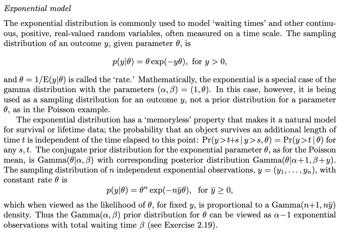
I think it did a pretty good job!

If you have a collection of scanned textbooks, this approach might be worth the 5 minutes it takes to set it up.