Don't know where your data is from? Bayesian modeling for unknown coordinates

An especially strong motivating case for the usage of spatial probability models comes from the mining industry. During exploration for mineral resources, prospectors will take geologic samples by drilling holes and examining the resulting material for presence or concentration of valuable ores. These data typically show strong spatial correlation, but constructing a fully-detailed geophysical model is at times infeasible as we are able to observe very little of the underground conditions, though the advent of remote sensing techniques like ground-penetrating radar and gravimetry has dramatically improved our ability to characterize Earth’s subsurface. To address this challenge, we would like to construct a probability model which uses nearby data to predict a variable of interest at a new location.

To illustrate the problem better, we will use a dataset of uranium and vanadium point-referenced concentration measurements from Walker Lake. The data originate from Isaaks and Srivastava’s An Introduction to Applied Geostatistics and are distributed with the R package gstat.

Up to this point, you may have seen lots of examples of how Gaussian process models are use in robotics, spatial statistics, neuroscience, etc. Now, we work through a more exotic example which modifies the Gaussian process model to accommodate the case in which the actual location of our data points is not known precisely, and is only observed with substantial measurement noise. Spatial location error changes the covariance and prediction problem itself, a point emphasized in geostatistical work on location error and GP regression work on noisy spatial inputs by Cressie and Kornak and Cervone and Pillai.

This may seem like an unusual example at first glance, but we include it to give an example of how Bayesian modeling with appropriate priors lets us modify and change nearly any part of the model, given that we have some idea of how to represent our assumptions as part of the model process. Then, we use Monte Carlo methods to turn the inference crank and obtain reliable parameter estimates.

Introducing some more notation, let \(\tilde{\mathbf{s}}_i\) denote the recorded coordinate and \(\mathbf{s}_i\) the latent coordinate where the measurement actually occurred. We use \(\mathbf{s}_i = \tilde{\mathbf{s}}_i + \Delta_i\), with \(\Delta_i \sim \operatorname{Normal}(\mathbf{0}, \sigma_s^2 I_2)\), and evaluate the Gaussian process at \(\mathbf{s}_i\) rather than at \(\tilde{\mathbf{s}}_i\). Our choice of coordinate system here is somewhat arbitrary; we could also choose to work with polar coordinates and place priors over the magnitude and the angle of the location error. The scale \(\sigma_s\) is treated as known in this example so that the model represents different assumed levels of coordinate error.

\[\begin{aligned} \Delta_i &\sim \mathrm{Normal}(\mathbf{0}, \sigma_s^2\mathbf{I}_2) \\ \mathbf{s}_i &= \tilde{\mathbf{s}}_i + \Delta_i \\ \mu &\sim \mathrm{Normal}(2, 2) \\ \sigma &\sim \mathrm{HalfNormal}(1) \\ \ell &\sim \mathrm{HalfNormal}(100) \\ \sigma_0 &\sim \mathrm{HalfNormal}(0.5) \\ f(\cdot) \mid \sigma,\ell &\sim \mathcal{GP}(0, \sigma^2 c(\cdot,\cdot;\ell)) \\ Y_i \mid f,\mu,\sigma_0,\mathbf{s}_i &\sim \mathrm{Normal}(\mu + f(\mathbf{s}_i), \sigma_0) \end{aligned}\]

This model is computationally harder than the fixed-location GP because the covariance matrix changes whenever the latent coordinates change. We use pm.gp.Marginal so that the latent GP values at the observations are integrated out.

We will construct datasets with increasing noise and examine how the model’s parameter estimates change. To begin, we perturb the original coordinates with increasing noise:

from pathlib import Path

import arviz as az
import matplotlib as mpl
import matplotlib.pyplot as plt
import numpy as np
import pandas as pd
import pymc as pm
import seaborn as sns
from matplotlib import colors
from matplotlib.patches import Circle

from stsp import use_sepia_gunmetal

RANDOM_SEED = 8927
np.random.seed(RANDOM_SEED)

theme, sepia_cmap = use_sepia_gunmetal()

plot_bg_color = "#1c1c1d"
plot_text_color = "#e8e8e8"

plt.style.use("dark_background")
mpl.rcParams.update(
    {
        "figure.facecolor": plot_bg_color,
        "axes.facecolor": plot_bg_color,
        "savefig.facecolor": plot_bg_color,
        "savefig.edgecolor": plot_bg_color,
        "text.color": plot_text_color,
        "axes.labelcolor": plot_text_color,
        "xtick.color": plot_text_color,
        "ytick.color": plot_text_color,
        "axes.edgecolor": "#828282",
    }
)

theme["paper"] = plot_bg_color

df = pd.read_csv(Path("../../data/walker/cleaned.csv"))

X_walker = df[["x_m", "y_m"]].to_numpy()
y_walker = df["u_log10_p1"].to_numpy()

n_prediction_grid = 70
buffer_fraction = 0.1
x_range = df["x_m"].max() - df["x_m"].min()
y_range = df["y_m"].max() - df["y_m"].min()
x_limits = (df["x_m"].min() - buffer_fraction * x_range, df["x_m"].max() + buffer_fraction * x_range)
y_limits = (df["y_m"].min() - buffer_fraction * y_range, df["y_m"].max() + buffer_fraction * y_range)
x_new = np.linspace(*x_limits, n_prediction_grid)
y_new = np.linspace(*y_limits, n_prediction_grid)
x_new_mesh, y_new_mesh = np.meshgrid(x_new, y_new)
Xnew = np.column_stack([x_new_mesh.ravel(), y_new_mesh.ravel()])

eps = np.random.randn(*X_walker.shape)
multipliers = [12.0, 25.0, 40.0]
noisy_xs = [X_walker + m * eps for m in multipliers]

The perturbed coordinates are shown in Figure X. We keep the target variable unchanged in this analysis. Next, we construct the model, using the pm.Data object as a container to let us swap out coordinates easily.

location_coords = {"obs": np.arange(X_walker.shape[0]), "coord": ["x", "y"]}
selected_location_idx = np.sort(np.random.default_rng(RANDOM_SEED).choice(X_walker.shape[0], size=4, replace=False))
location_error_idatas = {}

with pm.Model(coords=location_coords) as location_error_gp_model:
    X_noisy = pm.Data("X_noisy", noisy_xs[0], dims=("obs", "coord"))
    y = pm.Data("y", y_walker, dims="obs")
    σ_s = pm.Data("σ_s", multipliers[0])

    Δs = pm.Normal("Δs", 0.0, σ_s, dims=("obs", "coord"))
    X_true = pm.Deterministic("X_true", X_noisy + Δs, dims=("obs", "coord"))

    μ = pm.Normal("μ", 2.0, 2.0)
    σ = pm.HalfNormal("σ", 1.0)
    ℓ = pm.HalfNormal("ℓ", 100.0)
    σ0 = pm.HalfNormal("σ0", 0.5)

    cov = σ**2 * pm.gp.cov.Matern52(2, ls=ℓ)
    gp_location = pm.gp.Marginal(mean_func=pm.gp.mean.Constant(μ), cov_func=cov)
    gp_location.marginal_likelihood("y_obs", X=X_true, y=y, sigma=σ0, dims="obs")

    for multiplier, X_noisy_value in zip(multipliers, noisy_xs):
        pm.set_data({"X_noisy": X_noisy_value, "σ_s": multiplier})
        location_error_idatas[multiplier] = pm.sample(
            chains=2,
            cores=2,
            target_accept=0.95,
            mp_ctx="spawn",
            random_seed=RANDOM_SEED,
            progressbar=False,
        )

location_error_parameter_summaries = {
    multiplier: az.summary(idata, var_names=["μ", "σ", "ℓ", "σ0"])
    for multiplier, idata in location_error_idatas.items()
}
location_error_diagnostics = pd.DataFrame(
    [
        {
            "Location error SD": multiplier,
            "Divergences": int(idata.sample_stats["diverging"].sum()),
            "Max $\\hat{R}$": location_error_parameter_summaries[multiplier]["r_hat"].max(),
            "Min bulk ESS": location_error_parameter_summaries[multiplier]["ess_bulk"].min(),
            "Mean displacement": np.sqrt((idata.posterior["Δs"] ** 2).sum("coord")).mean().item(),
        }
        for multiplier, idata in location_error_idatas.items()
    ]
)
location_error_diagnostics

Initializing NUTS using jitter+adapt_diag...
Multiprocess sampling (2 chains in 2 jobs)
NUTS: [Δs, μ, σ, ℓ, σ0]
Sampling 2 chains for 1_000 tune and 1_000 draw iterations (2_000 + 2_000 draws total) took 6340 seconds.
There were 24 divergences after tuning. Increase `target_accept` or reparameterize.
Chain 1 reached the maximum tree depth. Increase `max_treedepth`, increase `target_accept` or reparameterize.
We recommend running at least 4 chains for robust computation of convergence diagnostics
The rhat statistic is larger than 1.01 for some parameters. This indicates problems during sampling. See https://arxiv.org/abs/1903.08008 for details
The effective sample size per chain is smaller than 100 for some parameters.  A higher number is needed for reliable rhat and ess computation. See https://arxiv.org/abs/1903.08008 for details
Initializing NUTS using jitter+adapt_diag...
Multiprocess sampling (2 chains in 2 jobs)
NUTS: [Δs, μ, σ, ℓ, σ0]
Sampling 2 chains for 1_000 tune and 1_000 draw iterations (2_000 + 2_000 draws total) took 6376 seconds.
There were 79 divergences after tuning. Increase `target_accept` or reparameterize.
Chain 0 reached the maximum tree depth. Increase `max_treedepth`, increase `target_accept` or reparameterize.
We recommend running at least 4 chains for robust computation of convergence diagnostics
The rhat statistic is larger than 1.01 for some parameters. This indicates problems during sampling. See https://arxiv.org/abs/1903.08008 for details
The effective sample size per chain is smaller than 100 for some parameters.  A higher number is needed for reliable rhat and ess computation. See https://arxiv.org/abs/1903.08008 for details
Initializing NUTS using jitter+adapt_diag...
Multiprocess sampling (2 chains in 2 jobs)
NUTS: [Δs, μ, σ, ℓ, σ0]
Sampling 2 chains for 1_000 tune and 1_000 draw iterations (2_000 + 2_000 draws total) took 7756 seconds.
There were 52 divergences after tuning. Increase `target_accept` or reparameterize.
Chain 0 reached the maximum tree depth. Increase `max_treedepth`, increase `target_accept` or reparameterize.
Chain 1 reached the maximum tree depth. Increase `max_treedepth`, increase `target_accept` or reparameterize.
We recommend running at least 4 chains for robust computation of convergence diagnostics
The rhat statistic is larger than 1.01 for some parameters. This indicates problems during sampling. See https://arxiv.org/abs/1903.08008 for details
The effective sample size per chain is smaller than 100 for some parameters.  A higher number is needed for reliable rhat and ess computation. See https://arxiv.org/abs/1903.08008 for details

	Location error SD	Divergences	Max \(\hat{R}\)	Min bulk ESS	Mean displacement
0	12.0	24	1.00	268.0	15.280551
1	25.0	79	1.03	126.0	31.874539
2	40.0	52	1.02	44.0	51.138540

location_surface_grids = {}
with location_error_gp_model:
    for multiplier, X_noisy_value in zip(multipliers, noisy_xs):
        pm.set_data({"X_noisy": X_noisy_value, "σ_s": multiplier})
        posterior_mean_point = {
            name: location_error_idatas[multiplier].posterior[name].mean(("chain", "draw")).values
            for name in ["μ", "σ", "ℓ", "σ0", "Δs", "X_true"]
        }
        f_mean, _ = gp_location.predict(Xnew, point=posterior_mean_point, diag=True, pred_noise=False)
        location_surface_grids[multiplier] = f_mean.reshape(n_prediction_grid, n_prediction_grid)

naive_kde_grids = {}
kde_bandwidths = {
    multiplier: location_error_idatas[multiplier].posterior["ℓ"].mean(("chain", "draw")).item()
    for multiplier in multipliers
}
for multiplier, X_noisy_value in zip(multipliers, noisy_xs):
    squared_distance = (
        (Xnew[:, 0, None] - X_noisy_value[:, 0]) ** 2
        + (Xnew[:, 1, None] - X_noisy_value[:, 1]) ** 2
    )
    weights = np.exp(-0.5 * squared_distance / kde_bandwidths[multiplier]**2)
    naive_kde_grids[multiplier] = (weights @ y_walker / weights.sum(axis=1)).reshape(n_prediction_grid, n_prediction_grid)

location_norm = colors.Normalize(
    vmin=min(y_walker.min(), *(grid.min() for grid in location_surface_grids.values())),
    vmax=max(y_walker.max(), *(grid.max() for grid in location_surface_grids.values())),
)
point_colors = [theme["gunmetal"], theme["sepia"], theme["rust"], theme["steel"]]
arrow_head_width = 0.018 * max(x_range, y_range)

fig = plt.figure(figsize=(5, 11.2 * (5 / 7)))
gs = fig.add_gridspec(4, len(multipliers), hspace=0.08, wspace=0.08)
axes = np.array([[fig.add_subplot(gs[row, col]) for col in range(len(multipliers))] for row in range(4)])
panel_idx = 0
surface_meshes = []

for col, (multiplier, X_noisy_value) in enumerate(zip(multipliers, noisy_xs)):
    ax = axes[0, col]
    ax.scatter(X_walker[:, 0], X_walker[:, 1], facecolor=theme["paper"], edgecolor=theme["gunmetal"], s=14, linewidth=0.35, alpha=0.5)
    ax.scatter(X_noisy_value[:, 0], X_noisy_value[:, 1], c=y_walker, cmap=sepia_cmap, norm=location_norm, s=16, edgecolor=theme["paper"], linewidth=0.25, alpha=0.5)
    for point_idx, point_color in zip(selected_location_idx, point_colors):
        circle = Circle(X_noisy_value[point_idx], radius=multiplier, facecolor=colors.to_rgba(theme["steel"], 0.2), edgecolor=theme["gunmetal"], linewidth=0.6)
        ax.add_patch(circle)
        dx, dy = X_noisy_value[point_idx] - X_walker[point_idx]
        ax.arrow(X_walker[point_idx, 0], X_walker[point_idx, 1], dx, dy, color=plot_text_color, linewidth=0.8, length_includes_head=True, head_width=arrow_head_width, head_length=arrow_head_width)
    ax.scatter(X_walker[selected_location_idx, 0], X_walker[selected_location_idx, 1], facecolor=theme["paper"], edgecolor=plot_text_color, s=44, linewidth=0.8)
    ax.scatter(X_noisy_value[selected_location_idx, 0], X_noisy_value[selected_location_idx, 1], c=y_walker[selected_location_idx], cmap=sepia_cmap, norm=location_norm, s=44, edgecolor=plot_text_color, linewidth=0.8)
    ax.xaxis.set_label_position("top"); ax.set_xlabel(rf"$\sigma_s = {multiplier:.0f}$ m")

    ax = axes[2, col]
    mesh = ax.pcolormesh(x_new_mesh, y_new_mesh, location_surface_grids[multiplier], cmap=sepia_cmap, norm=location_norm, shading="auto")
    surface_meshes.append(mesh)

    ax = axes[3, col]
    ax.pcolormesh(x_new_mesh, y_new_mesh, naive_kde_grids[multiplier], cmap=sepia_cmap, norm=location_norm, shading="auto")

    ax = axes[1, col]
    ax.pcolormesh(x_new_mesh, y_new_mesh, location_surface_grids[multiplier], cmap=sepia_cmap, norm=location_norm, shading="auto", alpha=0.25)
    X_true_samples = location_error_idatas[multiplier].posterior["X_true"].stack(sample=("chain", "draw")).transpose("obs", "coord", "sample")
    for point_idx, point_color in zip(selected_location_idx, point_colors):
        x_draws = X_true_samples.isel(obs=point_idx).sel(coord="x").values
        y_draws = X_true_samples.isel(obs=point_idx).sel(coord="y").values
        sns.kdeplot(x=x_draws, y=y_draws, levels=3, color=point_color, linewidths=0.9, fill=False, ax=ax)
        ax.scatter(X_walker[point_idx, 0], X_walker[point_idx, 1], marker="x", color=point_color, s=34, linewidth=1.1)
        ax.scatter(X_noisy_value[point_idx, 0], X_noisy_value[point_idx, 1], marker="o", facecolor=theme["paper"], edgecolor=point_color, s=34, linewidth=1.1)

for row, row_label in enumerate(["Perturbed coordinates", "Posterior location density", r"Posterior mean of $f(s)$", "Naive smoothed KDE"]):
    axes[row, 0].set_ylabel(row_label)

for ax in axes.ravel():
    ax.set_xlim(*x_limits); ax.set_ylim(*y_limits); ax.set_aspect("equal"); ax.grid(False)
    ax.tick_params(axis="both", which="both", bottom=False, left=False, top=False, right=False, labelbottom=False, labelleft=False, labeltop=False, labelright=False)
    panel_idx += 1

cbar = fig.colorbar(surface_meshes[-1], ax=axes.ravel().tolist(), orientation="horizontal", fraction=0.035, pad=0.04)
cbar.set_label(r"Uranium, $\log_{10}(x + 1)$")

figure_dir = Path.home() / "ckrapu.github.io/images/2026-05-24-dont-know-where-your-data-is-from"
figure_dir.mkdir(parents=True, exist_ok=True)
fig.savefig(figure_dir / "error-in-location-grid.png", dpi=220, bbox_inches="tight", facecolor=fig.get_facecolor())

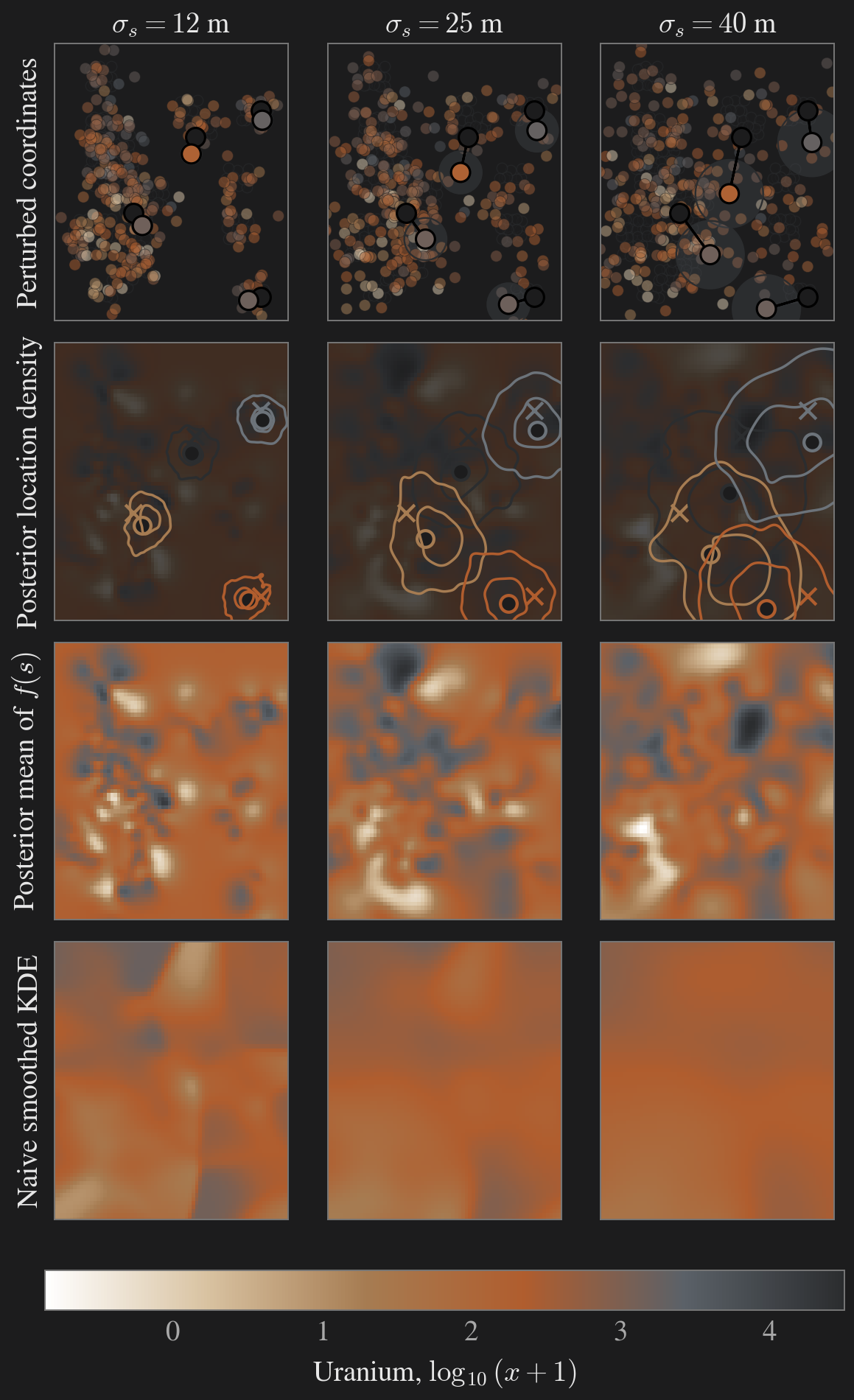
Figure 6 Data and posterior inference for a GP model with point coordinates which are only approximately observed. The top row shows the true, original coordinates in hollow circles while the noisily observed data points are shaded according to the uranium concentration at that point. The larger circles indicate the spatial scale of the coordinate error. The second row shows contours for the posterior high density region of the true location of four selected points in space; we see that as \(\sigma_s\) increases, these regions gracefully grow larger and larger.

As we examine Figure 6, we can see that some of the main features of the underlying surface are preserved even as the uncertainty in the coordinates grows. We see a few lighter features in the lower left corner, and a darker region in the top left and lower right. There is variation across these, but it is impressive that we can even work at all with this data given the severity of the perturbations! We include a comparison using a simpler approach, the Nadaraya-Watson Gaussian kernel smoother, with its bandwidth set to match the posterior mean estimate of the length scale under each scenario, and we find that it is unable to provide more than a rough average with little capacity to represent spatial variation.

Enjoy Reading This Article?