Simulating planetary waves

Rossby waves, also known as planetary waves, are large-scale waves that occur in the atmosphere and oceans of planets due to the variation of the Coriolis effect with latitude. On Earth, these waves are a fundamental component of atmospheric and oceanic circulation, playing a crucial role in transporting heat, momentum, and moisture across the globe. They are responsible for many of the large-scale weather patterns we experience, including the formation and movement of high and low-pressure systems, which dictate storm tracks and temperature extremes. Understanding Rossby waves is essential for predicting weather systems and analyzing long-term climate variability.

This notebook aims to demonstrate how to perform a series of simplified models for understanding and visualizing these waves. We will start with basic analytical solutions and progress towards more complex simulations to explore their behavior and characteristics.

We’ll start by setting up the key parameters for our simulation. These parameters are fundamental to defining the environment and conditions under which the Rossby waves will be modeled. They include spatial dimensions such as the size of the domain in both the x and y directions, which will represent a portion of the Earth’s surface. We also define the grid resolution by specifying the number of grid cells in each direction, nx and ny, which directly impacts the level of detail captured in the simulation and the computational cost.

The time parameters, such as max_time_s and the number of iterations, determine the duration of the simulation and the frequency at which we observe the wave’s evolution. We set the angular velocity, omega_rad_s, which is the physical property driving the Coriolis effect, a fundamental force behind the generation and behavior of Rossby waves.

import numpy as np
import tqdm
import scipy
import matplotlib.pyplot as plt
import warnings

from matplotlib.animation import FuncAnimation
from IPython.display import HTML, clear_output
import matplotlib as mpl
from dataclasses import dataclass

plt.style.use('dark_background')

# Numpy complains when we use .real on a complex-valued array, so
# we suppress that warning to keep the notebook short.
warnings.filterwarnings('ignore', category=np.exceptions.ComplexWarning)

Our first version of this will be simplified to use a Cartesian coordinate system roughly matching Earth’s parameters, with a rectangular domain as wide and tall as half the Earth’s circumference, and with an angular velocity roughly matching our own.

Note that the role of the omega_rad_s is only to impart accelerations due to the Coriolis effect. The root cause of planetary waves is the differing strength of the Coriolis affect across latitudes.

@dataclass
class SimulationConfig():
  '''
  Values and parameters which won't be changing during the simulation runs.
  '''
  omega_rad_s = 7.29e-5
  earth_radius_m = 6_371_000
  U = 50 # Average zonal velocity, in meters / s
  x_size_m = 40_075_000 / 2
  y_size_m = 40_075_000 / 2
  nx = 100 # number of grid cells in horizontal direction
  ny = 100 # number of grid cells vertically
  dx = x_size_m / nx
  dy = y_size_m / ny
  max_time_s = 3600*24*30 # in terms of seconds, hours, and days
  iterations = 300
  timesteps = np.linspace(0, max_time_s, iterations)

  # separate 2d arrays where each element contains the x- or y-location of
  # that grid cell
  x_arr, y_arr = np.meshgrid(
      np.linspace(0, x_size_m, nx),
      np.linspace(0, y_size_m, ny)
  )

  # We also need the latitude values for each grid cell,
  # in units of radians
  latitude_arr  = y_arr / y_size_m * np.pi / 2
  beta_arr = 2 * omega_rad_s * np.cos(latitude_arr) / earth_radius_m

cfg = SimulationConfig()

Run Rossby wave simulation

The explanations in this section are based on the Wikipedia page for planetary waves where you can learn more about their derivation. Note that this section mixes both Cartesian (\(x,y\)) and polar (\(\phi\)) coordinates. To reconcile this, we only use the polar c

Our first version of this will be simplified to use a Cartesian coordinate system, which is a two-dimensional flat grid, as opposed to a spherical coordinate system that would more accurately represent the Earth’s curved surface. The rectangular domain used here roughly matches the scale of half the Earth’s circumference in both width and height. The angular velocity parameter is set to a value that approximates Earth’s rotational rate.

Note that the role of the omega_rad_s is primarily to impart accelerations due to the Coriolis effect, which is a fictitious force observed in a rotating frame of reference that deflects moving objects. The root cause of planetary waves, however, is not the Coriolis effect itself, but rather the differing strength of the Coriolis effect across latitudes. This variation is known as the beta effect, and it is this latitudinal gradient that provides the restoring force for Rossby waves, causing them to propagate westward relative to the mean flow. In a Cartesian system, the beta effect is often introduced as a linear variation of the Coriolis parameter with the y-coordinate (representing latitude). The resulting PDE is:

where \(U\) denotes the average zonal velocity, also described as the mean westerly flow. Note that \(\beta = \frac{2\omega \cos \phi}{a}\), the Rossby parameter, captures the dependence of the system on latitude, as well as the size of the Earth and the speed of Earth’s rotation.

Our first version will use an analytical solution, specified in terms of Cartesian coordinates \(x\), \(y\), wavenumbers \(k\) and \(l\), and angular velocity \(\omega\). The analytical solution provides a direct mathematical expression for the streamfunction \(\psi(x,y,t)\) as a function of spatial position \((x, y)\) and time \(t\).

Here, \(\psi_0\) represents the amplitude of the wave, and \(k\) and \(l\) are the zonal and meridional wavenumbers, respectively. Wavenumbers describe the spatial frequency of the wave in the x and y directions. A larger wavenumber corresponds to a shorter wavelength and finer spatial structure. The term \(\omega t\) represents the temporal evolution of the wave, with \(\omega\) being the angular frequency of the wave. Note that a realistic solution for atmospheric or oceanic flows would typically involve the superposition of many such terms with different wavenumbers and amplitudes, representing a spectrum of waves. This simulation, for simplicity, uses a combination of a few selected wavenumbers to illustrate the basic wave behavior. Our simulation logic tracks the values of the streamfunction \(\psi\) over time and space. The streamfunction itself is a scalar field, but its gradient \(\nabla \psi\) is physically meaningful as it represents the velocity field of the underlying fluid. Specifically, in this simplified model, the velocity components \((u, v)\) are given by \(u = -\partial\psi / \partial y\) and \(v = \partial\psi / \partial x\). Therefore, we also calculate and store the gradient of the streamfunction in both the x and y directions throughout the simulation.

A realistic solution would involve the superposition of terms from multiple wavenumbers. This simulation just uses a few of them. Our simulation logic tracks the values of the streamfunction \(\psi\) as well as its gradient, as the velocity of the underlying fluid field is specified in terms of the gradient \(\nabla \psi\).

@dataclass
class SimulationState():
  '''
  Contains the state variables for the simulation.
  '''
  ψ: np.ndarray
  u: np.ndarray
  v: np.ndarray

state = SimulationState(
  ψ = np.zeros((cfg.iterations, cfg.ny, cfg.nx)),
  u = np.zeros((cfg.iterations, cfg.ny, cfg.nx)),
  v = np.zeros((cfg.iterations, cfg.ny, cfg.nx))
)

def rossby_wave(x, y, ω, t, ψ_0, k, l):
  '''
  Copied from https://en.wikipedia.org/wiki/Rossby_wave#Free_barotropic_Rossby_waves_under_a_zonal_flow_with_linearized_vorticity_equation
  '''

  return ψ_0 * np.exp(1j * (k * x + l * y - ω * t))

def omega(k, l):
  return cfg.U*k - cfg.beta_arr * k / (k**2 + l**2)

# Wavenumbers for the Rossby waves
# Define wavenumbers in physical units (rad/m)
k_physical = 2 * np.pi / (10000e3)  # 10,000 km wavelength
l_physical = 2 * np.pi / (8000e3)   # 8,000 km wavelength

# Convert to grid units
ks = [k_physical * n for n in range(1, 3)] # zonal
ls = [l_physical] # meriodonal

# Note that only the gradient of the streamfunction is physically meaningful
# so this parameter is unimportant for the simulation.
ψ_0 = 1.0


with tqdm.tqdm(total=cfg.iterations, desc="Simulating Rossby waves") as pbar:
  for i, t in enumerate(cfg.timesteps):
    current_ψ = ψ_0 * sum(
        rossby_wave(cfg.x_arr, cfg.y_arr, omega(k, l), t, ψ_0, k, l) for k in ks for l in ls
    )
    state.ψ[i] = current_ψ
    grady, gradx = np.gradient(ψ[i], cfg.dy, cfg.dx)
    state.v[i] = gradx   # -∂ψ/∂y (eastward velocity)
    state.u[i] = - grady # ∂ψ/∂x (northward velocity)

    # Calculate RMS average of the streamfunction
    rms_psi = np.sqrt(np.mean(np.abs(current_ψ)**2))
    pbar.set_description("RMS(ψ): {:.2f}".format(rms_psi))
    pbar.update(1)

Make single plot of wave at final timestep

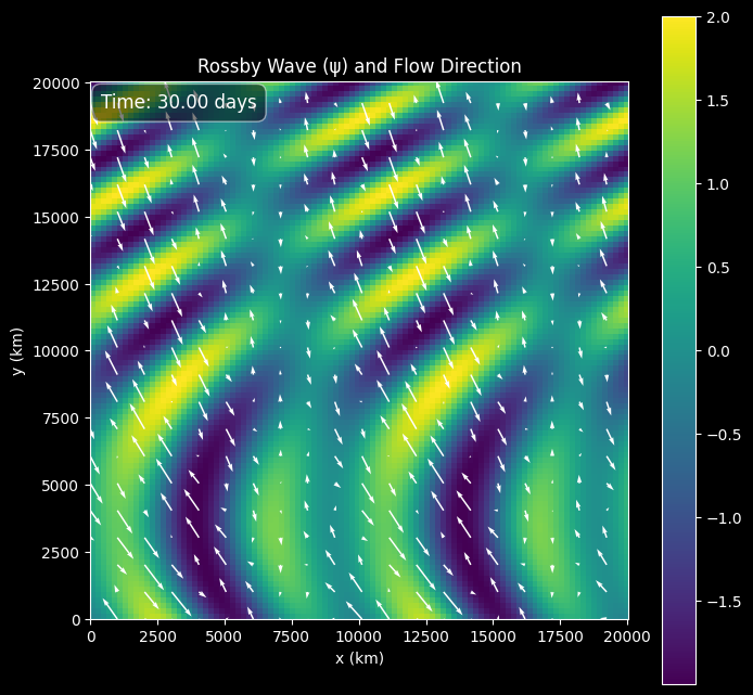
Let’s visualize a single timestep from the simulation to understand the spatial structure of the Rossby wave and the associated fluid motion. Here, the color intensity represents the real part of the streamfunction \(\psi\) at the last calculated timestep, providing a spatial map of this scalar field across the domain. Areas of high \(\psi\) are shown in warmer colors, while areas of low \(\psi\) are in cooler colors. The white arrows, displayed using a quiver plot, indicate the direction and magnitude of the gradient of the streamfunction, \(\nabla \psi\), at various points across the grid.

As discussed earlier, the gradient of the streamfunction is directly related to the velocity field of the underlying fluid. Specifically, in a 2D incompressible flow represented by a streamfunction, the velocity components \((u, v)\) are given by \(u = -\partial\psi / \partial y\) and \(v = \partial\psi / \partial x\). Therefore, the arrows show the instantaneous velocity vectors \((u, v)\) at each location, revealing the instantaneous flow direction and speed. High values of \(\psi\) often correspond to regions of anticyclonic (clockwise in the Northern Hemisphere) circulation, while low values correspond to cyclonic (counter-clockwise in the Northern Hemisphere) circulation. The arrows show the fluid parcel trajectories at this specific moment in time, revealing the large-scale circulation patterns driven by the wave.

fig, ax = plt.subplots()

# Remember that imshow doesn't know the x-y coords for this data;
# we have to give it the extent.
im = ax.imshow(state.ψ[-1].real, origin='lower', extent=[0, cfg.x_size_m/1000, 0, cfg.y_size_m/1000])
plt.colorbar(im, label = "Streamfunction $$\psi(x,y)$$")
plt.ylabel("y (km)"), plt.xlabel('x (km)')

# Since the grid is quite large, we subset the locations in which we actually
# place arrows using the quiver plot. Picking the right `n` is mostly just trial
# and error.
n = 5
q = ax.quiver(cfg.x_arr[::n, ::n]/1000, cfg.y_arr[::n, ::n]/1000, state.u[-1, ::n, ::n], state.v[-1, ::n, ::n],
  color='w')
ax.set_aspect('equal', adjustable='box') # Ensure aspect ratio is equal

Animating the streamfunction and velocity field

To appreciate the dynamical nature of the Rossby wave and observe its characteristic westward propagation, we can create an animation showing its evolution over the course of the simulated period, which spans several days. While the static plot provides a snapshot at a single moment, the animation reveals how the wave structure, represented by the streamfunction contours and the associated velocity field, changes and moves over time. As the animation progresses through the timesteps, we can see the crests and troughs of the streamfunction pattern propagating across the domain.

# Create animation of ψ over time using matplotlib and func animation. Show the animation here

# Increase the animation embed limit
mpl.rcParams['animation.embed_limit'] = 50.0  # Increase the limit to 50 MB

fig, ax = plt.subplots(figsize=(8, 8)) # Create a single figure and axes

# Plot for ψ (heatmap)
im = ax.imshow(np.real(state.ψ[0]), origin='lower', extent=[0, cfg.x_size_m/1000, 0, cfg.y_size_m/1000])
plt.colorbar(im, ax=ax)
ax.set_title('Rossby Wave (ψ) and Flow Direction')
ax.set_xlabel('x (km)')
ax.set_ylabel('y (km)')


# Add a text annotation for time
time_text = ax.text(0.02, 0.95, '', transform=ax.transAxes, color='white', fontsize=12,
                    bbox=dict(boxstyle='round,pad=0.5', fc='black', alpha=0.5))

# Plot for gradient (quiver)
# We need to subsample the grid for the quiver plot to avoid overcrowding
step = 5 # Adjust this value to change the density of arrows
quiver_plot = ax.quiver(cfg.x_arr[::step, ::step]/1000, cfg.y_arr[::step, ::step]/1000,
                         state.u[0, ::step, ::step], state.v[0, ::step, ::step],
                         color='white')
ax.set_aspect('equal', adjustable='box')


def animate(i):
    im.set_data(np.real(state.ψ[i]))
    time_in_days = cfg.timesteps[i] / (3600 * 24)
    time_text.set_text(f'Time: {time_in_days:.2f} days')

    quiver_plot.set_UVC(state.u[i, ::step, ::step], state.v[i, ::step, ::step])
    return [im, time_text, quiver_plot]

ani = FuncAnimation(fig, animate, frames=cfg.iterations, interval=50, blit=True)

HTML(ani.to_html5_video())