A tutorial on kinematics and optimization using NVIDIA Warp
Warp is a promising new open-source software library for performing scientific computing and optimization on GPUs with a Python-native workflow.
This notebook provides a simple first example of using Warp to simulate a particle moving along a one-dimensional flow field. We’ll then optimize the direction and magnitude of the flow field to push the particle towards a pair of target locations specified at two distinct timesteps. It doesn’t assume much background in fluid mechanics or machine learning, and shows the basic workflow for manipulating the parameters of a simulation using Warp.
Simulating a particle’s movement in 1D
We start by importing packages and defining the simulation parameters. For the purposes of this project, Warp can be considered as a drop-in replacement for PyTorch or Jax - it includes both the tensor libraries and automatic differentiation logic.
from dataclasses import dataclass
from IPython.display import HTML
from matplotlib.animation import FuncAnimation
from tqdm import tqdm
from IPython.display import Image

import matplotlib as mpl
import matplotlib.pyplot as plt
import numpy as np
import warp as wp

plt.style.use('dark_background')

plot_bg_color = "#1c1c1d"

mpl.rcParams['figure.facecolor'] = plot_bg_color
mpl.rcParams['axes.facecolor'] = plot_bg_color

np.random.seed(8271991)

device = "cuda"

# Instantiate a variable to force Warp to start up
# and show its version + device
wp.array([0], dtype=float, device=device)
array(shape=(1,), dtype=float32)
Here, we specify that the domain will be one meter long and divided into 100 grid cells for numerical simulation. The entire simulation will run for 30 seconds in increments of 100 milliseconds.
@dataclass
class ParticleExampleConfig:
    length_m: float = 1.0
    nx: int = 100
    total_time_s: float = 30.
    dt: float = 0.1
    start_location_m = 0.1

particle_cfg = ParticleExampleConfig()
Next, we define the logic for tracking the location of the particle as it is moved around via the velocity field.
def simulate_particle(particle_cfg: ParticleExampleConfig, u0: wp.array) -> wp.array:
      '''
      Runs a simple 1D simulation, taking the flow field (a 1D vector in this case) and produces
      an array with the location of the particle at each timestep.
      '''
      n_steps = int(particle_cfg.total_time_s / particle_cfg.dt)
      positions = wp.zeros(n_steps + 1, dtype=wp.float32, requires_grad=True)

      @wp.kernel
      def integrate_trajectory(
          positions: wp.array(dtype=wp.float32),
          u0: wp.array(dtype=wp.float32),
          start_pos: float,
          dt: float,
          dx: float,
          nx: int,
          n_steps: int
      ):
          tid = wp.tid()

          if tid == 0:
              positions[0] = start_pos
              velocity = float(0.0)

              for step in range(n_steps):
                  current_pos = positions[step]

                  cell_idx = wp.int32(current_pos / dx)
                  cell_idx = wp.clamp(cell_idx, 0, nx - 1)

                  flow_velocity = u0[cell_idx]
                  force = flow_velocity - velocity

                  velocity = velocity + force * dt

                  new_pos = current_pos + velocity * dt
                  new_pos = wp.clamp(new_pos, 0.0, dx * float(nx))

                  positions[step + 1] = new_pos

      dx = particle_cfg.length_m / particle_cfg.nx

      wp.launch(
          integrate_trajectory,
          dim=1,
          inputs=[
              positions,
              u0,
              particle_cfg.start_location_m,
              particle_cfg.dt,
              dx,
              particle_cfg.nx,
              n_steps
          ]
      )

      return positions
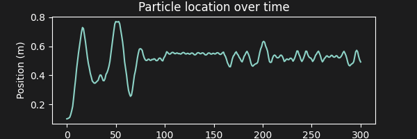
Let’s go ahead and run it, with a velocity field which is randomly initialized but with a bias pointing towards the center of the domain.
u0_numpy = np.random.randn(particle_cfg.nx) + np.linspace(1, -1, particle_cfg.nx) * 2.5
u0 = wp.array(u0_numpy, dtype=float, device=device)
positions = simulate_particle(particle_cfg, u0)

plt.figure(figsize=(6, 2))
plt.xlabel("Time (s)"), plt.ylabel("Position (m)")
plt.title("Particle location over time")
plt.plot(positions.numpy())
plt.savefig("visuals/location_over_time.png")
plt.close()
Image("visuals/location_over_time.png")
We can also make an animation to provide a dynamic view of the particle’s behavior subject to the 1D velocity field.
fig, ax = plt.subplots(figsize=(8, 2))

ax.set_xlim(0, particle_cfg.length_m)
ax.set_ylim(-0.5, 0.5)
ax.set_xlabel("Position (m)")

# Turn off y-axis + spines
ax.axes.get_yaxis().set_visible(False)
for spine in ['top', 'right', 'left']:
    ax.spines[spine].set_visible(False)

# Add tight layout to prevent xlabel cutoff
plt.tight_layout()

particle = ax.scatter([], [], s=100, color='cyan')
time_text = ax.text(0.02, 0.85, '', transform=ax.transAxes, fontsize=10)

# Get position data
positions_np = positions.numpy()
n_frames = len(positions_np)

def init():
    particle.set_offsets(np.empty((0, 2)))
    time_text.set_text('')
    return particle, time_text

def animate(frame):
    particle.set_offsets([[positions_np[frame], 0]])
    time_text.set_text(f'Time: {frame * particle_cfg.dt:.1f}s')

    return particle, time_text

anim = FuncAnimation(fig, animate, init_func=init,
                    frames=n_frames, interval=40,
                    blit=True, repeat=True)
anim.save('visuals/01-position-animation.gif', writer='pillow', fps=25, dpi=80)
HTML(anim.to_jshtml())
Great! We’ve got a simple model for a particle moving subject to a velocity field. Let’s move onto the meat of this tutorial - manipulating the model parameters to do what we want.
Optimizing the velocity field via automatic differentiation
We’ve passed an initial test of basic functionality for our model; we assume a simple velocity field and let the particle be moved around subject to simple kinematics.
Next, we want to show how to optimize an arbitrary model quantity to perform an interesting task. Our new objective is to identify a setting of u0 that pushes the particle to a target location at a given timestep. Our optimization strategy is as follows:
For each iteration:
- We take the initial velocity field
u0which is just a 1D array for this problem, and run the forward simulation. We use thetapeto record the execution trace - Next, we use reverse-mode autodiff in Warp to get
gradwhich represents \(\nabla_{u_0} L(x_1,...,x_T)\) where \(x_1,...,x_T\) denotes the particle position at each timestep. - We apply an update to
u0per the update rule \(u_0^{(i+1)} = u_0^{(i)} - \eta ^{(i)} \cdot \nabla_{u_0^{i}} \left[ L(x_1^{(i)},...,x_T^{(i)}) \right]\) with \(u_0^{(i+1)}\) as the value of the velocity field at the \(i+1\)-th iteration and \(x_1^{(i-1)}\) denoting the value of the position of the particle at timestep 1 in optimization iteration \(i-1\). Our loss function \(L\) is simply the sum of the squared distances between the position locations and the target locations at the provided timesteps. - We decrease the update size with \(\eta ^{(i+1)} = \eta ^{(i)} \times 0.99\)
'''
The configs for this version are mostly the same; we just want
to include a few validation checks.
'''

@dataclass
class ParticleOptimizationConfig(ParticleExampleConfig):
    target_times_s: tuple[float] = (1., 15.)
    target_locations_m: tuple[float] = (0.2, 0.75)
    step_size = 0.1
    n_iterations = 25
    decay_rate = 0.99 # Decreases the step size by this factor each iteration

    def __post_init__(self):
        if len(self.target_times_s) != len(self.target_locations_m):
            raise ValueError("target_times_s and target_locations_m must have the same length.")
        if any(t < 0 or t > self.total_time_s for t in self.target_times_s):
            raise ValueError("All target times must be within the total simulation time.")
        if any(l < 0 or l > self.length_m for l in self.target_locations_m):
            raise ValueError("All target locations must be within the simulation length.")

opt_cfg = ParticleOptimizationConfig()
Applying autodiff and gradient descent
The above configuration specifies that at 1 and 15 seconds in simulation time we would like the particle to be close to locations of 0.2 m and 0.75 m from the left-hand side of the domain. We’ll use Warp’s implementation of automatic differentiation with gradient descent and a simple decreasing stepsize schedule to find an optimal u0 such that the particle respects the previous conditions.
u0_history = []
u0 = wp.array(np.random.randn(opt_cfg.nx) * 0.1, dtype=wp.float32, device=device, requires_grad=True)

target_indices = [int(t / opt_cfg.dt) for t in opt_cfg.target_times_s]
target_positions = wp.array(opt_cfg.target_locations_m, dtype=wp.float32, device=device)

loss_history = []
grad_norm_history = []

pbar = tqdm(range(opt_cfg.n_iterations), desc="")
step_size = opt_cfg.step_size

for iteration in pbar:
    u0_history.append(u0.numpy().copy())

    tape = wp.Tape()

    with tape:
        positions = simulate_particle(opt_cfg, u0)

        loss = wp.zeros(1, dtype=wp.float32, device=device, requires_grad=True)

        @wp.kernel
        def compute_l2_loss(
            positions: wp.array(dtype=wp.float32),
            target_positions: wp.array(dtype=wp.float32),
            target_indices: wp.array(dtype=wp.int32),
            loss: wp.array(dtype=wp.float32)
        ):
            tid = wp.tid()
            if tid <= target_indices.shape[0]:
                idx = target_indices[tid]
                diff = positions[idx] - target_positions[tid]
                wp.atomic_add(loss, 0, diff * diff)

        target_indices_array = wp.array(target_indices, dtype=wp.int32, device=device)
        wp.launch(compute_l2_loss, dim=len(target_indices),
                 inputs=[positions, target_positions, target_indices_array, loss])

    tape.backward(loss)

    loss_val = loss.numpy()[0]
    grad = tape.gradients[u0].numpy()
    grad_norm = np.linalg.norm(grad)

    loss_history.append(loss_val)
    grad_norm_history.append(grad_norm)

    pbar.set_description(f"Iter {iteration}: Loss = {loss_val:.6f}, Grad norm = {grad_norm:.6f}")

    u0_np = u0.numpy()
    u0_np -= opt_cfg.step_size * grad
    u0 = wp.array(u0_np, dtype=wp.float32, device=device, requires_grad=True)

    step_size *= opt_cfg.decay_rate
Iter 24: Loss = 0.000754, Grad norm = 0.028800: 100%|██████████| 25/25 [00:00<00:00, 156.56it/s]

Module __main__ 331110c load on device 'cuda:0' took 0.20 ms  (cached)
Animating the optimized trajectory
Our optimization converges to near-zero loss quite quickly. Let’s see what the solution looks like:
optimized_positions = simulate_particle(opt_cfg, u0)

fig, ax = plt.subplots(figsize=(8, 2))

ax.set_xlim(0, opt_cfg.length_m)
ax.set_ylim(-0.5, 0.5)
ax.set_xlabel("Position (m)")

ax.axes.get_yaxis().set_visible(False)
for spine in ['top', 'right', 'left']:
    ax.spines[spine].set_visible(False)

plt.tight_layout()

particle = ax.scatter([], [], s=100, color='cyan')
time_text = ax.text(0.02, 0.85, '', transform=ax.transAxes, fontsize=10)

for t, loc in zip(opt_cfg.target_times_s, opt_cfg.target_locations_m):
    ax.axvline(x=loc, color='cyan', linestyle='--', alpha=0.5)
    ax.text(loc, 0.3, f't={t}s', ha='center', fontsize=8, color='cyan')

positions_np = optimized_positions.numpy()
n_frames = len(positions_np)

def init():
    particle.set_offsets(np.empty((0, 2)))
    time_text.set_text('')
    return particle, time_text

def animate(frame):
    particle.set_offsets([[positions_np[frame], 0]])
    time_text.set_text(f'Time: {frame * opt_cfg.dt:.1f}s')

    return particle, time_text

anim = FuncAnimation(fig, animate, init_func=init,
                    frames=n_frames, interval=40,
                    blit=True, repeat=True)
anim.save('visuals/01-optimize-animation.gif', writer='pillow', fps=25, dpi=80)
HTML(anim.to_jshtml())
To understand how the solution evolves over iterations, let’s animate the particle movement for several values of u0 obtained at the start, middle, and end of optimization.
n_rows, n_cols = 2, 6

n_subplots = n_rows * n_cols
step = max(1, opt_cfg.n_iterations // n_subplots)
selected_iterations = list(range(0, opt_cfg.n_iterations, step))[:n_subplots]

fig, axes = plt.subplots(n_rows, n_cols, figsize=(16, n_rows*1.5))
axes = axes.flatten()

for i, ax in enumerate(axes):
    ax.set_xlim(0, opt_cfg.length_m)
    ax.set_ylim(-0.5, 0.5)
    ax.set_xticks([0, 0.5, 1.0])
    ax.tick_params(labelsize=8)

    ax.axis('off')

plt.tight_layout()

particles = []
titles = []

for i, (ax, iter_idx) in enumerate(zip(axes, selected_iterations)):
    particle = ax.scatter([], [], s=50, color='cyan', edgecolor='w')
    particles.append(particle)


    title = ax.text(0.05, 0.9, f'Iter. {iter_idx}', transform=ax.transAxes,
                   ha='center', fontsize=11, color='white')
    titles.append(title)

    for t, loc in zip(opt_cfg.target_times_s, opt_cfg.target_locations_m):
        ax.axvline(x=loc, color='cyan', linestyle='--', alpha=0.2, linewidth=3.0)

def init():
    for particle in particles:
        particle.set_offsets(np.empty((0, 2)))
    return particles

def animate(frame):
    frame = frame * 2

    for i, (particle, iter_idx) in enumerate(zip(particles, selected_iterations)):
        u0_iter = wp.array(u0_history[iter_idx], dtype=wp.float32, device=device)
        positions = simulate_particle(opt_cfg, u0_iter)
        positions_np = positions.numpy()

        if frame < len(positions_np):
            particle.set_offsets([[positions_np[frame], 0]])

    return particles

n_frames = int(opt_cfg.total_time_s / opt_cfg.dt) + 1
anim = FuncAnimation(fig, animate, init_func=init,
                    frames=n_frames//2, interval=80,
                    blit=True, repeat=True)
anim.save('visuals/01-history-animation.gif', writer='pillow', fps=25, dpi=80)
HTML(anim.to_jshtml())
Enjoy Reading This Article?
Here are some more articles you might like to read next: